During the first weeks as a GSoC 2022 contributor for FEniCS, I have developed a demo showing how to implement scattering boundary conditions in FEniCSx. In particular, I have used scattering boundary conditions for simulating the scattering of a TM-polarized plane wave by an infinite gold wire.

Scattering from a wire with scattering boundary conditions

This demo is implemented in three files: one for the mesh generation with gmsh, one for the calculation of analytical results, and one for the variational forms and the solver. The demo illustrates how to:

• Use complex quantities in FEniCSx
• Setup and solve Maxwell’s equations
• Implement scattering boundary conditions
• Calculate analytical and numerical efficiencies for scattering problems

Equations, problem definition and implementation

First of all, let’s import the modules that will be used:

import gmsh
import numpy as np
from gmsh_helpers import gmsh_model_to_mesh
from mesh_wire import generate_mesh_wire
import pyvista
import ufl
from dolfinx import fem, plot
from ufl import (FacetNormal, as_vector, conj, cross, curl, inner, lhs, rhs,
                 sqrt)
from scipy.special import h2vp, hankel2, jv, jvp
from mpi4py import MPI
from petsc4py import PETSc

Since we want to solve Maxwell’s equation, we need to specify that the demo should only be executed with DOLFINx complex mode, otherwise it would not work:

if not np.issubdtype(PETSc.ScalarType, np.complexfloating):
    print("Demo should only be executed with DOLFINx complex mode")
    exit(0)

Now, let’s consider an infinite metallic wire immersed in a background medium (e.g. vacuum or water) that is hit by an electromagnetic wave with its wavevector and electric field perpendicular to the wire axis. Due to the degeneracy of the problem along the axis direction, we can solve the problem in two-dimension, with our domain being $\Omega=\Omega_{m} \cup\Omega_{b}$, made up by the cross-section of the wire $\Omega_m$ and the background medium $\Omega_{b}$ surrounding the wire. We will delimit our domain with an external circular boundary $\partial \Omega$. Our aim is to calculate the electric field $\mathbf{E}_s$ scattered by the wire. We will consider a background plane wave with a wavelength $\lambda_0$. Mathematically, we can write:

with $\mathbf{k} = \frac{2\pi}{\lambda_0}n_b\hat{\mathbf{u}}_k$ being the wavevector of the plane wave, pointing along the propagation direction, with $\hat{\mathbf{u}}_p$ being the polarization direction, and with $\mathbf{r}$ being a point in $\Omega$. We will only consider $\hat{\mathbf{u}}_k$ and $\hat{\mathbf{u}}_p$ with components belonging to the $\Omega$ domain and perpendicular to each other, i.e. $\hat{\mathbf{u}}_k \perp \hat{\mathbf{u}}_p$ (transversality condition of plane waves). If we call $x$ and $y$ the horizontal and vertical axis in our $\Omega$ domain, and by defining $k_x = n_bk_0\cos\theta$ and $k_y = n_bk_0\sin\theta$, with $\theta$ being the angle defined by the propagation direction $\hat{\mathbf{u}}_k$ and the horizontal axis $\hat{\mathbf{u}}_x$, we can write more explicitly:

The BackgroundElectricField class below implements such function. The inputs to the function are the angle $\theta$, the background refractive index $n_b$ and the vacuum wavevector $k_0$. The function returns the expression $\mathbf{E}_b = -\sin \theta e^{j (k_xx+k_yy)}\hat{\mathbf{u}}_x + \cos\theta e^{j (k_xx+k_yy)}\hat{\mathbf{u}}_y$.

class BackgroundElectricField:

    def __init__(self, theta, n_b, k0):
        self.theta = theta
        self.k0 = k0
        self.n_b = n_b

    def eval(self, x):

        kx = self.n_b * self.k0 * np.cos(self.theta)
        ky = self.n_b * self.k0 * np.sin(self.theta)
        phi = kx * x[0] + ky * x[1]

        ax = np.sin(self.theta)
        ay = np.cos(self.theta)

        return (-ax * np.exp(1j * phi), ay * np.exp(1j * phi))

The Maxwell’s equation for scattering problems takes the following form:

where $k_0 = 2\pi/\lambda_0$ is the vacuum wavevector of the background field, $\varepsilon_b$ is the background relative permittivity and $\varepsilon_r$ is the relative permittivity as a function of space, i.e.:

with $\varepsilon_m$ being the relative permittivity of the metallic wire. As reference values, we will consider $\lambda_0 = 400\textrm{nm}$ (violet light), $\varepsilon_b = 1.33^2$ (relative permittivity of water), and $\varepsilon_m = -1.0782 + 5.8089\textrm{j}$ (relative permittivity of gold at $400\textrm{nm}$).

To make the system fully determined, we need to add some boundary conditions on $\partial \Omega$. A common approach is the use of scattering boundary conditions, which make the boundary transparent for $\mathbf{E}_s$, allowing us to restric the computational boundary to a finite $\Omega$ domain. The first-order boundary conditions in the 2D case take the following form:

with $n_b = \sqrt{\varepsilon_b}$ being the background refractive index, $\mathbf{n}$ being the normal vector to $\partial \Omega$, and $r = \sqrt{(x-x_s)^2 + (y-y_s)^2}$ being the distance of the $(x, y)$ point on $\partial\Omega$ from the wire centered in $(x_s, y_s)$. In our case we will consider the wire centered in the origin of our mesh, and therefore $r = \sqrt{x^2 + y^2}$.

Let’s therefore define the function $r(x)$ and the $\nabla \times$ operator for 2D vector, since they will be useful later on:

def radial_distance(x):
    """Returns the radial distance from the origin"""
    return ufl.sqrt(x[0]**2 + x[1]**2)


def curl_2d(a):
    """Returns the curl of two 2D vectors as a 3D vector"""
    ay_x = a[1].dx(0)
    ax_y = a[0].dx(1)
    return as_vector((0, 0, ay_x - ax_y))

Next we define some mesh specific parameters

# Constant definition
um = 10**-6  # micron
nm = 10**-9  # nanometer
pi = np.pi
epsilon_0 = 8.8541878128 * 10**-12
mu_0 = 4 * pi * 10**-7

# Radius of the wire and of the boundary of the domain
radius_wire = 0.050 * um
radius_dom = 1 * um

# The smaller the mesh_factor, the finer is the mesh
mesh_factor = 1.2

# Mesh size inside the wire
in_wire_size = mesh_factor * 7 * nm

# Mesh size at the boundary of the wire
on_wire_size = mesh_factor * 3 * nm

# Mesh size in the background
bkg_size = mesh_factor * 60 * nm

# Mesh size at the boundary
boundary_size = mesh_factor * 30 * nm

# Tags for the subdomains
au_tag = 1          # gold wire
bkg_tag = 2         # background
boundary_tag = 3    # boundary

We generate the mesh using GMSH and convert it to a dolfinx.mesh.Mesh.

model = generate_mesh_wire(
    radius_wire, radius_dom, in_wire_size, on_wire_size, bkg_size,
    boundary_size, au_tag, bkg_tag, boundary_tag)

mesh, cell_tags, facet_tags = gmsh_model_to_mesh(
    model, cell_data=True, facet_data=True, gdim=2)
gmsh.finalize()
MPI.COMM_WORLD.barrier()

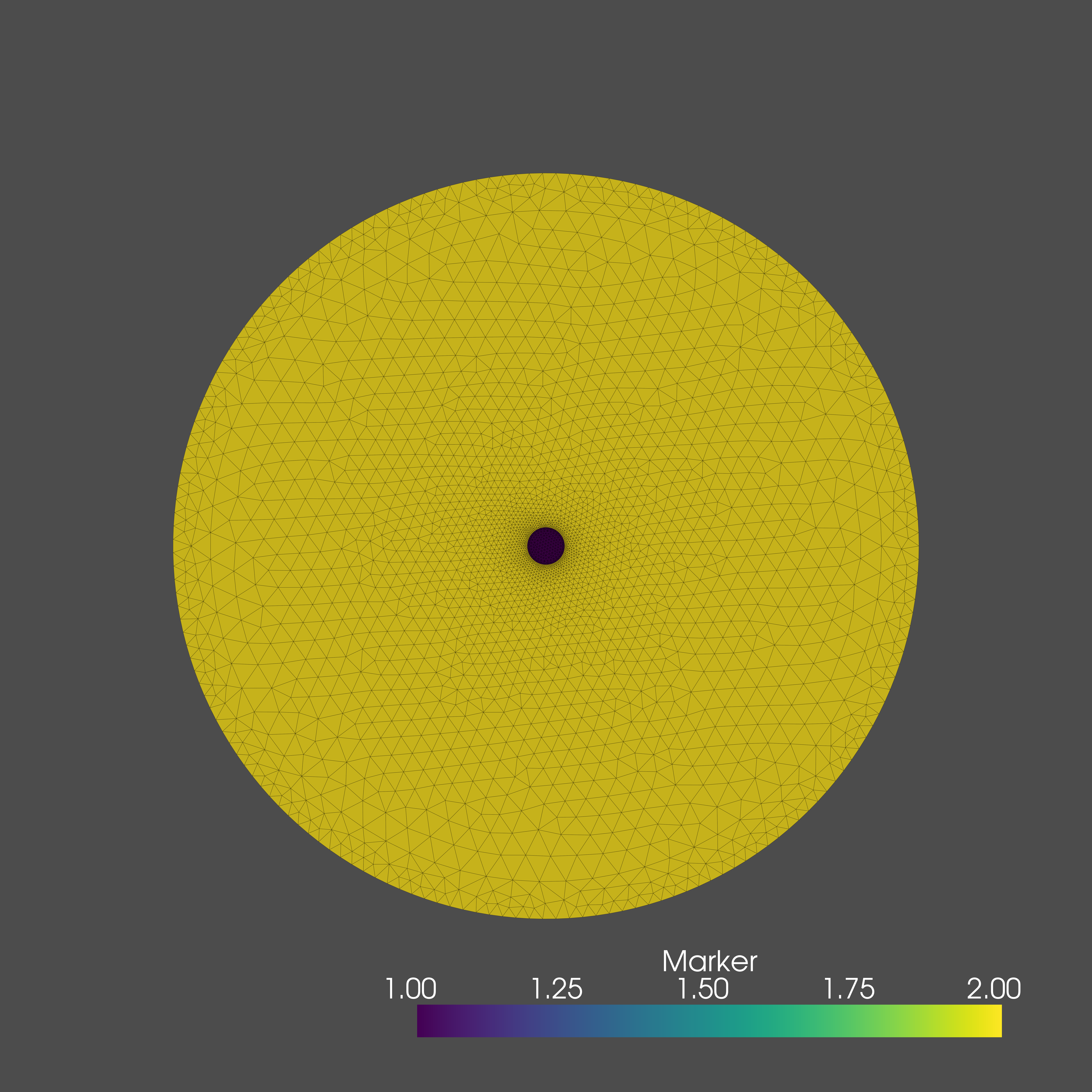
Let’s have a visual check of the mesh by plotting it with PyVista, by using different colors for cells with different tags: blue for the wire (au_tag) and yellow for the background medium (bkg_tag).

topology, cell_types, geometry = plot.create_vtk_mesh(mesh, 2)
grid = pyvista.UnstructuredGrid(topology, cell_types, geometry)
pyvista.set_jupyter_backend("pythreejs")
plotter = pyvista.Plotter()
num_local_cells = mesh.topology.index_map(mesh.topology.dim).size_local
grid.cell_data["Marker"] = cell_tags.values[cell_tags.indices<num_local_cells]
grid.set_active_scalars("Marker")
plotter.add_mesh(grid, show_edges=True)
plotter.view_xy()
if not pyvista.OFF_SCREEN:
    plotter.show()
else:
    pyvista.start_xvfb()
    figure = plotter.screenshot("wire_mesh.png")

The result is:

Now we define some other problem specific parameters:

wl0 = 0.4 * um  # Wavelength of the background field
n_bkg = 1.33 # Background refractive index
eps_bkg = n_bkg**2  # Background relative permittivity
k0 = 2 * np.pi / wl0  # Wavevector of the background field
deg = np.pi / 180
theta = 45 * deg  # Angle of incidence of the background field

and then the function space used for the electric field. We will use a 3rd order Nedelec (first kind) element:

degree = 3
curl_el = ufl.FiniteElement("N1curl", mesh.ufl_cell(), degree)
V = fem.FunctionSpace(mesh, curl_el)

Next, we can interpolate $\mathbf{E}_b$ into the function space $V$:

f = background_electric_field(theta, n_bkg, k0)
Eb = fem.Function(V)
Eb.interpolate(f.eval)

# Function r = radial distance from the (0, 0) point
x = ufl.SpatialCoordinate(mesh)
r = radial_distance(x)

# Definition of Trial and Test functions
Es = ufl.TrialFunction(V)
v = ufl.TestFunction(V)

# Definition of 3d fields for cross and curl operations
Es_3d = as_vector((Es[0], Es[1], 0))
v_3d = as_vector((v[0], v[1], 0))

# Measures for subdomains
dx = ufl.Measure("dx", mesh, subdomain_data=cell_tags)
ds = ufl.Measure("ds", mesh, subdomain_data=facet_tags)
dAu = dx(au_tag)
dBkg = dx(bkg_tag)
dDom = dAu + dBkg
dsbc = ds(boundary_tag)

# Normal to the boundary
n = FacetNormal(mesh)
n_3d = as_vector((n[0], n[1], 0))

Let’s now define the relative permittivity $\varepsilon_m$ of the gold wire at $400nm$ (data taken from Olmon et al. 2012):

# Definition of relative permittivity for Au @400nm
eps_au = -1.0782 + 1j * 5.8089

Now we can define a space function for the permittivity $\varepsilon$ that takes the value of the gold permittivity $\varepsilon_m$ for cells inside the wire, while it takes the value of the background permittivity $\varepsilon_b$ otherwise:

# Definition of the relative permittivity over the whole domain
D = fem.FunctionSpace(mesh, ("DG", 0))
eps = fem.Function(D)
au_cells = cell_tags.find(au_tag)
bkg_cells = cell_tags.find(bkg_tag)
eps.x.array[au_cells] = np.full_like(
    au_cells, eps_au, dtype=np.complex128)
eps.x.array[bkg_cells] = np.full_like(bkg_cells, eps_bkg, dtype=np.complex128)
eps.x.scatter_forward()

It is time to solve our problem, and therefore we need to find the weak form of the Maxwell’s equation plus with the scattering boundary conditions. As a first step, we need to take the inner products of the equations with a complex test function $\mathbf{v}$, and then we need to integrate the terms over the corresponding domains:

By using the $(\nabla \times \mathbf{A}) \cdot \mathbf{B}=\mathbf{A} \cdot(\nabla \times \mathbf{B})+\nabla \cdot(\mathbf{A} \times \mathbf{B})$ relation, we can change the first term into:

using the divergence theorem $\int_\Omega\nabla\cdot\mathbf{F}~\mathrm{d}x = \int_{\partial\Omega} \mathbf{F}\cdot\mathbf{n}~\mathrm{d}s$, we can write:

We can cancel $-(\nabla\times\mathbf{E}_s \times \bar{\mathbf{V}}) \cdot\mathbf{n}$ and $\mathbf{n} \times \nabla \times \mathbf{E}_s \cdot \bar{\mathbf{V}}$ thanks to the triple product rule $\mathbf{A} \cdot(\mathbf{B} \times \mathbf{C})=\mathbf{B} \cdot(\mathbf{C} \times \mathbf{A})=\mathbf{C} \cdot(\mathbf{A} \times \mathbf{B})$, arriving at the final weak form:

We can implement such equation in DOLFINx in the following way:

# Weak form
F = - inner(curl(Es), curl(v)) * dDom \
    + eps * k0 ** 2 * inner(Es, v) * dDom \
    + k0 ** 2 * (eps - eps_bkg) * inner(Eb, v) * dDom \
    + (1j * k0 * n_bkg + 1 / (2 * r)) \
    * inner(cross(Es_3d, n_3d), cross(v_3d, n_3d)) * dsbc

We can then split the weak form into its left-hand and right-hand side and solve the problem, by storing the scattered field $\mathbf{E}_s$ in Eh:

# Splitting in left-hand side and right-hand side
a, L = lhs(F), rhs(F)

problem = fem.petsc.LinearProblem(a, L, bcs=[], petsc_options={
                                  "ksp_type": "preonly", "pc_type": "lu"})
Eh = problem.solve()

Let’s now save the solution. To do so, we need to interpolate our solution discretized with Nedelec elements into a discontinuous Lagrange space, and then we can save the interpolated function as a .bp folder:

V_dg = fem.VectorFunctionSpace(mesh, ("DG", 3))
Esh_dg = fem.Function(V_dg)
Esh_dg.interpolate(Esh)

with VTXWriter(mesh.comm, "Esh.bp", Esh_dg) as f:
    f.write(0.0)

Next we can calculate the total electric field $\mathbf{E}=\mathbf{E}_s+\mathbf{E}_b$ and save it:

E = fem.Function(V)
E.x.array[:] = Eb.x.array[:] + Esh.x.array[:]

E_dg = fem.Function(V_dg)
E_dg.interpolate(E)

with VTXWriter(mesh.comm, "E.bp", E_dg) as f:
    f.write(0.0)

For more information about saving and visualizing vector fields discretized with Nedelec elements, check this DOLFINx demo. Instead of PyVista, we can also use ParaView for visualization and post-processing purposes. Here below an example of the time-harmonic evolution of $\operatorname{Re}(\mathbf{E})$ along $x$ obtained in ParaView (the field of view has been reduced for convenience):

If we are intereste in the norm of the electric field:

we can calculate it in DOLFINx in this way:

# ||E||
lagr_el = ufl.FiniteElement("CG", mesh.ufl_cell(), 2)
norm_func = sqrt(inner(Esh, Esh))
V_normEsh = fem.FunctionSpace(mesh, lagr_el)
norm_expr = fem.Expression(norm_func, V_normEsh.element.interpolation_points())
normEsh = fem.Function(V_normEsh)
normEsh.interpolate(norm_expr)

To validate our demo, we can compare our numerical results with analytical results. In particular, as reference quantities, we can consider the so-called absorption and scattering efficiencies. The analytical derivation of these quantities can be found at this reference. Here we will report the final result.

First of all, let’s define some parameters:

• $m = n/n_b$: relative refractive index of the wire,
• $r$: radius of the cross-section of the wire,
• $\alpha = 2\pi r n_b/\lambda_0$.

Now, let’s introduce the coefficients $a_l$ as:

where:

• $J_\nu(x)$: $\nu$-th order Bessel function of the first kind,
• $J_\nu^{\prime}(x)$: first derivative with respect to $x$ of the $\nu$-th order Bessel function of the first kind,
• $H_\nu^{(2)}(x)$: $\nu$-th order Hankel function of the second kind,
• $H_\nu^{(2){\prime}}(x)$: first derivative with respect to $x$ of the $\nu$-th order Hankel function of the second kind.

We have already imported these functions from scipy.special:

• jv(nu, x) ⟷ $J_\nu(x)$,
• jvp(nu, x, 1) ⟷ $J_\nu^{\prime}(x)$,
• hankel2(nu, x) ⟷ $H_\nu^{(2)}(x)$,
• h2vp(nu, x, 1) ⟷ $H_\nu^{(2){\prime}}(x)$.

The scattering, extinction and absorption efficiencies can be calculated as:

We can calculate these formula in Python with the below calculate_analytical_efficiencies function, having the following inputs:

• reps ⟷ $\operatorname{Re}(\varepsilon)$,
• ieps ⟷ $\operatorname{Im}(\varepsilon)$,
• n_bkg ⟷ $n_b$,
• wl0 ⟷ $\lambda_0$,
• radius_wire ⟷ $r$.

def calculate_analytical_efficiencies(reps, ieps, n_bkg, wl0, radius_wire):

    def a_coeff(nu, m, alpha):

        J_nu_alpha = jv(nu, alpha)
        J_nu_malpha = jv(nu, m * alpha)
        J_nu_alpha_p = jvp(nu, alpha, 1)
        J_nu_malpha_p = jvp(nu, m * alpha, 1)

        H_nu_alpha = hankel2(nu, alpha)
        H_nu_alpha_p = h2vp(nu, alpha, 1)

        a_nu_num = J_nu_alpha * J_nu_malpha_p - m * J_nu_malpha * J_nu_alpha_p
        a_nu_den = H_nu_alpha * J_nu_malpha_p - m * J_nu_malpha * H_nu_alpha_p

        return a_nu_num / a_nu_den

    m = np.sqrt(reps - 1j * ieps) / n_bkg

    alpha = 2 * np.pi * radius_wire / wl0 * n_bkg
    c = 2 / alpha

    num_n = 50

    for nu in range(0, num_n + 1):

        if nu == 0:

            q_ext = c * np.real(a_coeff(nu, m, alpha))
            q_sca = c * np.abs(a_coeff(nu, m, alpha))**2

        else:

            q_ext += c * 2 * np.real(a_coeff(nu, m, alpha))
            q_sca += c * 2 * np.abs(a_coeff(nu, m, alpha))**2

    q_abs = q_ext - q_sca

    return q_abs, q_sca, q_ext

Let’s run the function with our inputs:

q_abs_analyt, q_sca_analyt, q_ext_analyt = calculate_analytical_efficiencies(
    eps_au,
    n_bkg,
    wl0,
    radius_wire)

Now we can calculate the numerical efficiencies with the following formula:

with $Z_0 = \sqrt{\frac{\mu_0}{\varepsilon_0}}$ being the vacuum impedance, and with

being the scattered magnetic field. We can then normalize these values over the intensity of the electromagnetic field $I_0$ and the geometrical cross section of the wire, $\sigma_{gcs} = 2r_w$:

In FEniCSx, we can calculate these values in the following way:

# Vacuum impedance
Z0 = np.sqrt(mu_0 / epsilon_0)

# Magnetic field H
Hsh_3d = -1j * curl_2d(Esh) / Z0 / k0 / n_bkg

Esh_3d = as_vector((Esh[0], Esh[1], 0))
E_3d = as_vector((E[0], E[1], 0))

# Intensity of the electromagnetic fields I0 = 0.5*E0**2/Z0
# E0 = np.sqrt(ax**2 + ay**2) = 1, see background_electric_field
I0 = 0.5 / Z0

# Geometrical cross section of the wire
gcs = 2 * radius_wire

# Quantities for the calculation of efficiencies
P = 0.5 * inner(cross(Esh_3d, conj(Hsh_3d)), n_3d)
Q = 0.5 * np.imag(eps_au) * k0 * (inner(E_3d, E_3d)) / Z0 / n_bkg

# Define integration domain for the wire
dAu = dx(au_tag)

# Normalized absorption efficiency
q_abs_fenics_proc = (fem.assemble_scalar(fem.form(Q * dAu)) / gcs / I0).real
# Sum results from all MPI processes
q_abs_fenics = mesh.comm.allreduce(q_abs_fenics_proc, op=MPI.SUM)

# Normalized scattering efficiency
q_sca_fenics_proc = (fem.assemble_scalar(fem.form(P * dsbc)) / gcs / I0).real

# Sum results from all MPI processes
q_sca_fenics = mesh.comm.allreduce(q_sca_fenics_proc, op=MPI.SUM)

# Extinction efficiency
q_ext_fenics = q_abs_fenics + q_sca_fenics

Finally, we can evaluate the error, to validate our simulation:

# Error calculation
err_abs = np.abs(q_abs_analyt - q_abs_fenics) / q_abs_analyt
err_sca = np.abs(q_sca_analyt - q_sca_fenics) / q_sca_analyt
err_ext = np.abs(q_ext_analyt - q_ext_fenics) / q_ext_analyt

# Check if errors are smaller than 1%
assert err_abs < 0.01
assert err_sca < 0.01
assert err_ext < 0.01

if MPI.COMM_WORLD.rank == 0:

    print()
    print(f"The analytical absorption efficiency is {q_abs_analyt}")
    print(f"The numerical absorption efficiency is {q_abs_fenics}")
    print(f"The error is {err_abs*100}%")
    print()
    print(f"The analytical scattering efficiency is {q_sca_analyt}")
    print(f"The numerical scattering efficiency is {q_sca_fenics}")
    print(f"The error is {err_sca*100}%")
    print()
    print(f"The analytical extinction efficiency is {q_ext_analyt}")
    print(f"The numerical extinction efficiency is {q_ext_fenics}")
    print(f"The error is {err_ext*100}%")